
First, save the results of your simulation in Matlab format:
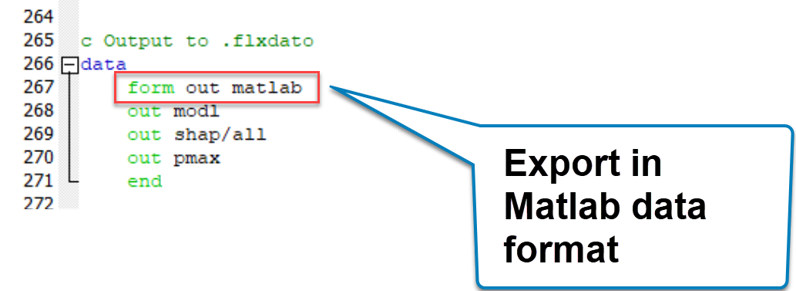
You will then obtain a "*.mat" format file that you can open with Python.
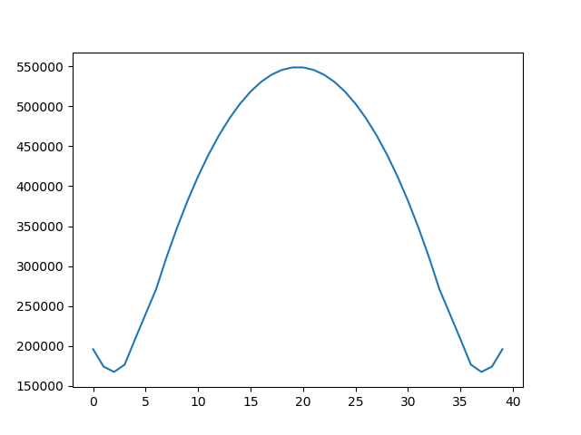
Example 1: Extracting apmx array from Onscale data and plotting a curve in Python from it
For example, here is a test result file in matlab format:
Download: pzt-simple-tuto-2d.mat
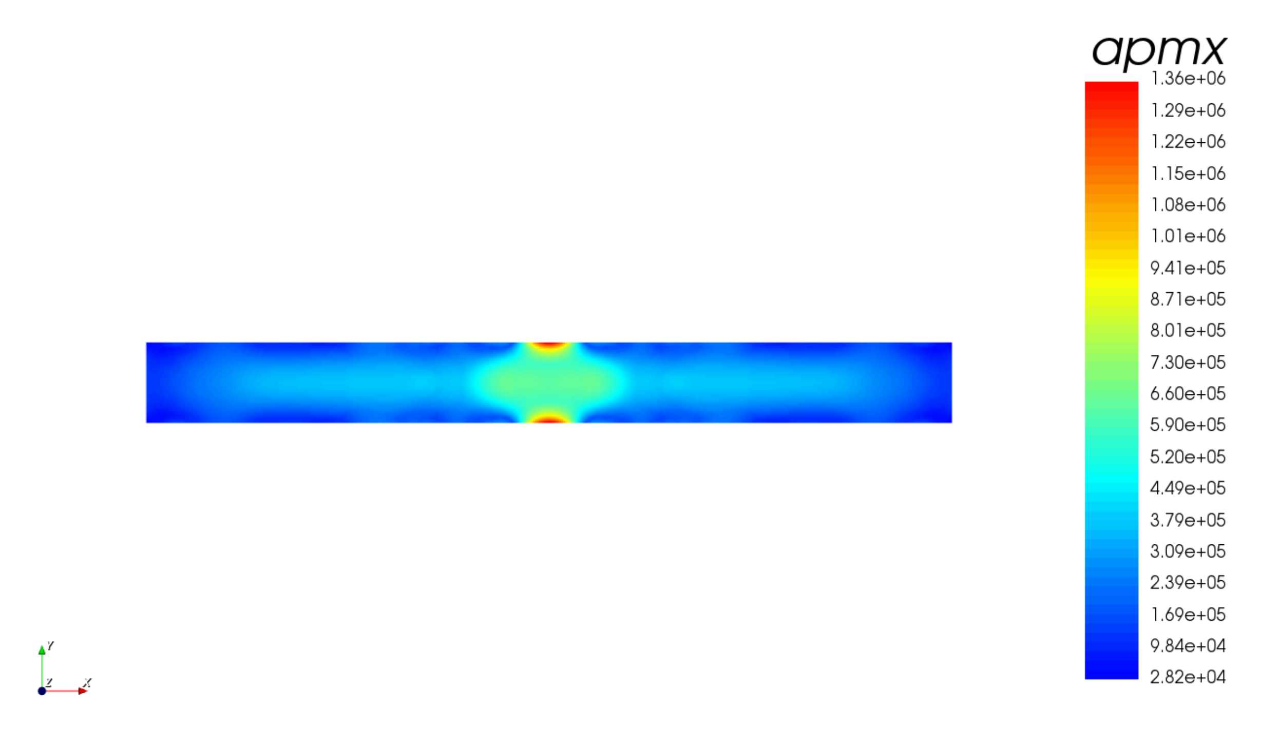
We will post-process with Python the data included in the apmx array (maximum acoustic pressure)
This is the apmx array vizualized in OnScale Post-process:
You can open and post-process it with the following Python Script
#!/usr/bin/python
import numpy as np
import matplotlib as ml
import matplotlib.pyplot as plt

from scipy.io import loadmat
x = loadmat('pzt-simple-tuto-2d.mat')

#Check the keys of the x array
print(x.keys())

#Extract the x and y coordinates
xcrd = x['d1_0006160_xcrd']
ycrd = x['d1_0006160_ycrd']


#Find the i value corresponding to a certain xval and save it to ival
xval = 150e-05

sampling = round(float(xcrd[2]-xcrd[1]),8)

for i in range(len(xcrd)):
    if(xval > xcrd[i]-sampling and xval < xcrd[i]+sampling):
        ival = i
print(ival)

#Plot the aprs in function of ival
plt.plot(x['d1_0006160_apmx'][ival])
plt.savefig('d1_0006160_apmx.png')
This python script postprocess the results and extract a curve at a position x = 150e-05
This is the resulting curve:
Note: You will need to install Python as well as numpy, matplotlib and scipy modules to follow this tutorial
Download the Python Script
Note: If you need more info about how to plot with matplotlib, check this page
Example 2: Plotting a 3D Interactive plot
It is possible to plot nice interactive 3D plot like this one too:
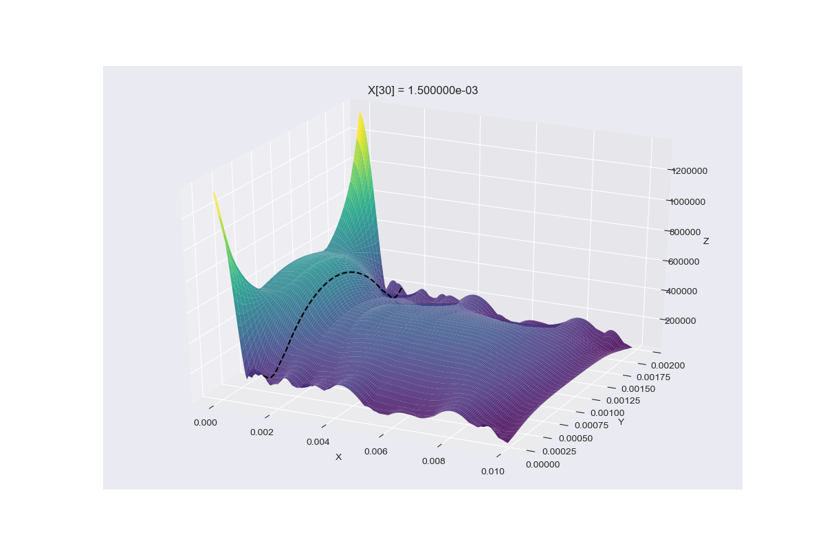
Here's the python code:
#!/usr/bin/env python
"""
    Demonstration of 3D post processing.
"""
import numpy as np
import matplotlib.pyplot as plt
from mpl_toolkits import mplot3d
from scipy.io import loadmat

plt.style.use('seaborn-darkgrid')

# Load Data
data = loadmat('pzt-simple-tuto-2d.mat')

# Extract (X, Y) coordinates. Cut off the final coord so shapes match.
X = data['d1_0006160_xcrd'].flatten()[:-1]
Y = data['d1_0006160_ycrd'].flatten()[:-1]


# The target X value we are looking for
x_val = 150e-05

# Find the index of this X value
dx = X[1] - X[0]
x_index = np.argmax((x_val > X - dx) & (x_val < X + dx))

# Create 3D coordinate grid
xx, yy = np.meshgrid(X, Y)

# Initialize figure
fig = plt.figure(figsize=(12, 8))
ax = plt.axes(projection='3d')

# Plot the apmx surface with some nice colors
zz = data['d1_0006160_apmx'].T
ax.plot_surface(xx, yy, zz, alpha=.9, rstride=1, cstride=1, cmap='viridis')

# Plot the 2D curve of our X value's cross-section slice
x = np.repeat(X[x_index], len(Y))
y = Y
z = zz[:, x_index]
ax.plot(x, y, z, color='k', ls='--', zorder=10)

# Label and display
ax.set_title("X[{:d}] = {:e}".format(x_index, X[x_index]))
ax.set_xlabel('X')
ax.set_ylabel('Y')
ax.set_zlabel('Z')
plt.show()