
OnScale integrates a new modal solver which is actually in Beta Testing Phase.
If you are interested to try it, I will detail briefly in this article how to structure your input file to calculate a number of modal frequencies and export the mode shape pictures.
Note: this modal solver is only available in Analyst Mode through script, it is not integrated yet in the Designer mode.
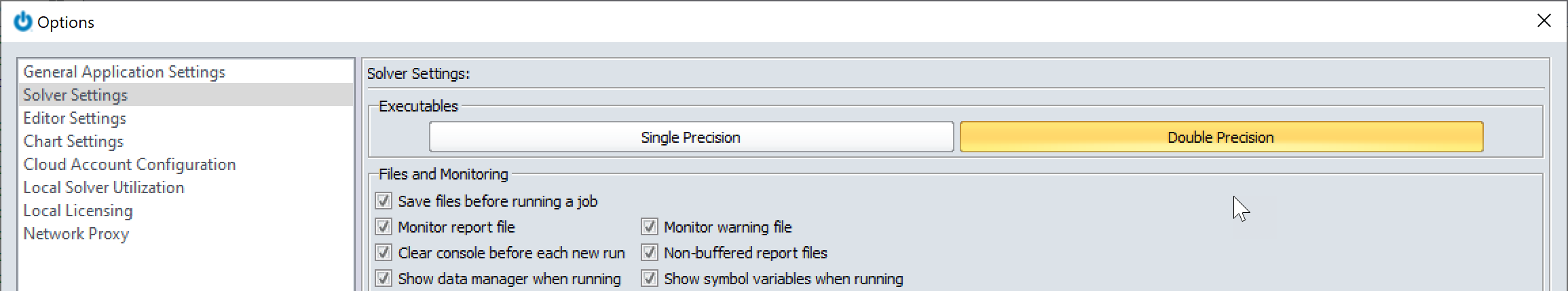
Important: Implicit mechanical requires double precision for reliable result
Because of that, you will need to go in the Options>Solver Settings and choose "Double Precision" for local run. If you are using the cloud, choose "Double Precision" when you run the script.
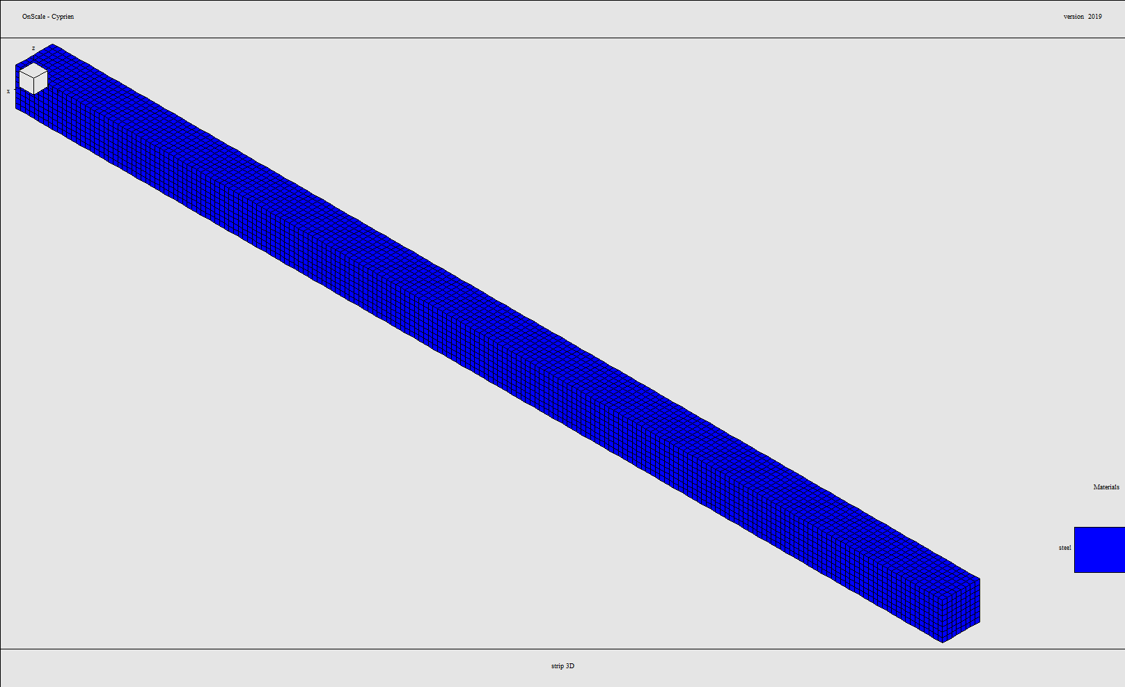
Example of Modal Analysis:
This is a very simple 3D model that you can use to test the modal solver:
Here is a sample code to run a modal analysis of a 3D Strip:
c mem 800 200 /* Allocate 800 megawords of memory - 3 GigaBytes (Not necesarry for Windows Operating Systems)
c NOTE: MEM Command must be first command in file, if used. (Line 1)
rest no

c *************************************************************************************************************
c
c 				Generated Flex Input File
c
c *************************************************************************************************************
c
c	DESIGNER			:OnScale - Designer Generated
c	MODEL DESCRIPTION	:
c	DATE CREATED		:11 Feb 2020
c	VERSION				:1.0
c
c	BASE UNITS			: kg-m-s
c	STRESS   			: Pa
c	FORCE    			: N
c *************************************************************************************************************

mp
	omp * *  		 /* Number of CPUs to be used in the execution.
	end

titl modal strip 3D

c *************************************************************************************************************
c
c 			Define User Variables
c
c *************************************************************************************************************
c
c These variables have been set by the user through the interface.
c
c *************************************************************************************************************
c Simulation Variables
symb AccelGrav       = 9.81  /* m/s^2
symb nbFreqs = 10 /* Number of Modes
symb neigar = 3 /* number of Arnoldi vectors
c
symb #get { JobName } jobname
text File_prcs = '$(JobName)_prcs.flxrsto'

symb coordFactor = 1.0		 /* Coordinate conversion factor
symb timeFactor = 1.0		 /* Time conversion factor
symb dMassFactor = 1.0		 /* Mass conversion factor

c *************************************************************************************************************
c
c             Define Materials
c
c *************************************************************************************************************
matr

c --------------------------------------------------------------
c type : MISC :
c name : steel :
c desc : Steel, generic :
c --------------------------------------------------------------
    wvsp off
    type elas
    prop steel 7700. 160.e9 80.e9 0.010000
    end

c *************************************************************************************************************
c
c 			Define Meshing
c
c *************************************************************************************************************
c
c 			Set the variable for the approximate element size for the model. Must be
c			sufficient to represent the wavelengths of interest. Recommended that at least
c			15 elements per wavelength are used.

c
c *************************************************************************************************************

symb box = 0.005	/* Size in X,Y Dir
symb box2 = 0.005 /* Size in Z Dir

c *************************************************************************************************************
c
c 			Geometry Locations (XYZ)
c
c *************************************************************************************************************


c Scale Parameters
symb xmin = 0.0 * $coordFactor
symb xmax = 0.04 * $coordFactor
symb ymin = 0.0 * $coordFactor
symb ymax = 0.4 * $coordFactor
symb zmin = 0.0 * $coordFactor
symb zmax = 0.04 * $coordFactor

c Determine lengths of the model
symb xlen = ( $xmax - $xmin )
symb ylen = ( $ymax - $ymin )
symb zlen = ( $zmax - $zmin )


c ***************************************************
c
c 			Keypoints in the X-Direction
c
c ***************************************************

symb #keycord x 1 $xmin $xlen
symb #get { idx } rootmax x

c ***************************************************
c
c 			Keypoints in the Y-Direction
c
c ***************************************************

symb #keycord y 1 $ymin $ylen
symb #get { jdx } rootmax y

c ***************************************************
c
c 			Keypoints in the Z-Direction
c
c ***************************************************

symb #keycord z 1 $zmin $zlen
symb #get { kdx } rootmax z

c *************************************************************************************************************
c
c 			Indices Locations (IJK)
c
c *************************************************************************************************************

c Grid in I direction, using approximately element size of 'box' and at least 1 element
symb #keyindx i 1 $idx 1 $box 1
symb indgrd = $i$idx

c Grid in J direction, using approximately element size of 'box' and at least 1 element
symb #keyindx j 1 $jdx 1 $box 1
symb jndgrd = $j$jdx

c Grid in K direction, using approximately element size of 'box' and at least 1 element
symb #keyindx k 1 $kdx 1 $box2 1
symb kndgrd = $k$kdx


c *************************************************************************************************************
c
c 			GCON Grid & Geometry Allocation
c
c *************************************************************************************************************

grid $i$idx $j$jdx $k$kdx
geom
	keypnt $idx $jdx $kdx
	end

c --------------------------------------------------------------
c                   Project Material List
c --------------------------------------------------------------


site
	regn void
	blok steel 0.0 0.04 0.0 0.4 0.0 0.04
	end

grph
	set imag png
	type standard
	line on
	plot matr
	imag model
	end

term

c *************************************************************************************************************
c
c 			Boundary Definitions
c
c *************************************************************************************************************

c grav 0 0 -$AccelGrav

boun
	side xmin free
	side xmax free
	side ymin fixd
	side ymax free
	side zmin free
	side zmax free
	end


c *************************************************************************************************************
c
c 			Calculated Properties
c
c *************************************************************************************************************
c
c 			By default, Flex only calculates the minimum required data set, typically this
c			means only velocities. This is done for memory efficiency. Should other
c			properites be required (e.g. displacements, stresses, strains, pressure), then
c			these must be requested by the CALC command. The manual lists all these options

c
c *************************************************************************************************************

calc
	disp x y z
	end


eign
	modes $nbFreqs 1 $neigar
	end

symb #msg 1
Checking Model Integrity......
prcs


grph
	type standard
	line on
	set imag png
	plot matr
	imag model.png
	end

c term


proc NormalizeDisps save
data
    symb #get { rMaxDisp } datamax tdsp
    symb ScaleFactor = 1. / $rMaxDisp * 0.05
    scal tdsp $ScaleFactor
    end
end$ proc

do loop1 I 1 $nbFreqs 1
eign
	modes $nbFreqs $I $neigar
	end

exec 1
calc
	vmag tdsp xdsp ydsp zdsp
	end

proc NormalizeDisps

grph
	type standard
	line on
	set imag png
	nvew 1 1
	disp $ScaleFactor
	plot tdsp
	imag mode_$I.png
	end

c term

end$ loop1


symb #msg 2 > 'freqs.txt'
Mode frequencies and relative residuals
 ---------------------------------------

do expFreqLoop I 1 $nbFreqs 1

symb #get { freq } arpack/d $I 1 1
symb #msg 1 >> 'freqs.txt'
Freq $I : $freq

end$ expFreqLoop
c *************************************************************************************************************
c
c 			Save modal frequencies to file for later use
c
c *************************************************************************************************************

symb #msg 2 > 'freqs.txt'
Mode frequencies and relative residuals
 ---------------------------------------

do expFreqLoop I 1 $nbFreqs 1

symb #get { freq } arpack/d $I 1 1
symb #msg 1 >> 'freqs.txt'
Freq_$I $freq

end$ expFreqLoop


c *************************************************************************************************************
c
c 			Save symbol variables to file for later use
c
c *************************************************************************************************************

symb #get { labl } jobname
symb #save '$labl.symb'
stop  		 /* return to command prompt
Results:
 Mode frequencies and relative residuals
 ---------------------------------------
               Col   1       Col   2
  Row   1:    2.08198D+02   1.12139D-15
  Row   2:    2.08198D+02   1.05739D-15
  Row   3:    1.24897D+03   9.84899D-17
  Row   4:    1.24897D+03   2.40239D-17
  Row   5:    1.83727D+03   1.58142D-17
  Row   6:    3.23913D+03   2.67841D-17
  Row   7:    3.29010D+03   1.39523D-17
  Row   8:    3.29010D+03   1.30021D-17
  Row   9:    5.51091D+03   5.44624D-17
  Row  10:    5.97917D+03   2.20058D-17
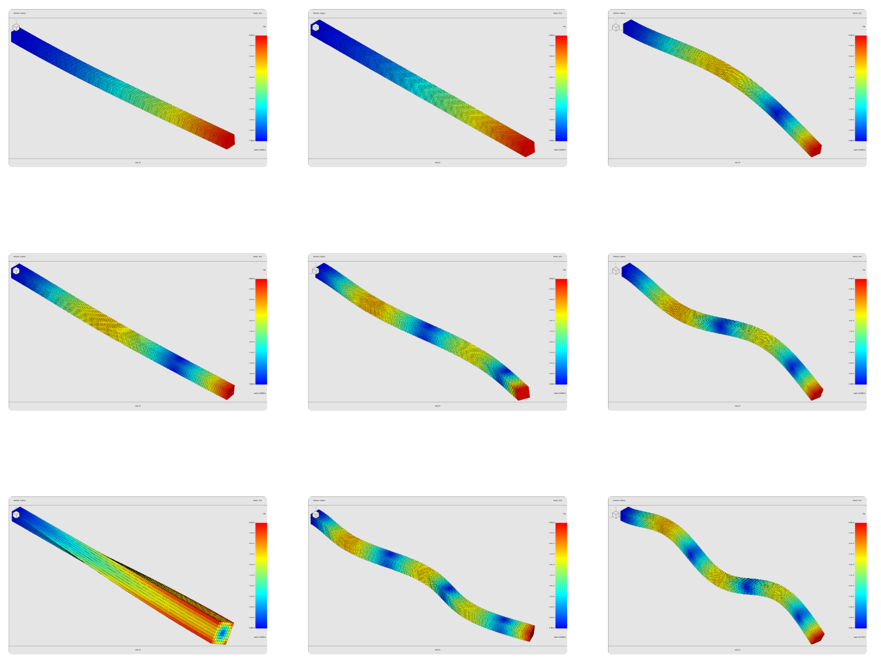
Modes Shapes:
Comparison with Theory (Roark's formula for stress and strain):
|
Kn |
fn (Hz) |
OnScale fn (Hz) |
Error |
|
3.51601527 |
51.01706952 |
51.02811 |
0.0216% |
|
22.0344915 |
319.7185161 |
317.7999 |
0.6037% |
|
61.6972144 |
895.2211052 |
881.1394 |
1.5981% |
|
120.901916 |
1754.276071 |
1702.803 |
3.0228% |
Explanations:
The way to use this solver is the following:
Use this new eign command after calc and before prcs
eign
                modes 10 1 3
                end
10: number of modes
1: mode shape requested
3: nb of arnoldi vectors ( for control of precision)
After that, use exec 1 to execute 1 step of calculation.
exec 1
Right after the exec:
calc
                vmag tdsp xdsp ydsp
grph
                type standard
                line on
                set imag png
                nvew 1 1
                disp 0.0000001
                plot tdsp
                imag mode_1.png
                end
vmag calculates total displacement array called tdsp from the xdsp and ydsp arrays.
grph will plot the mode shape requested
Note: Currently it is only possible to plot one mode shape at the time (second argument of “modes 10 1 3”). If you want all mode shapes, you have to use a loop like in the 3D strip example
You can then use the following code after the exec to write all the frequencies to a text file
symb #msg 2 > 'freqs.txt'
Mode frequencies and relative residuals
---------------------------------------

symb nbFreqs = 10

do expFreqLoop I 1 $nbFreqs 1

symb #get { freq } arpack/d $I 1 1
symb #msg 1 >> 'freqs.txt'
Freq $I : $freq

end$ expFreqLoop
The modal frequencies calculated are stored in the array arpack/d
(You can see it in the data manager)
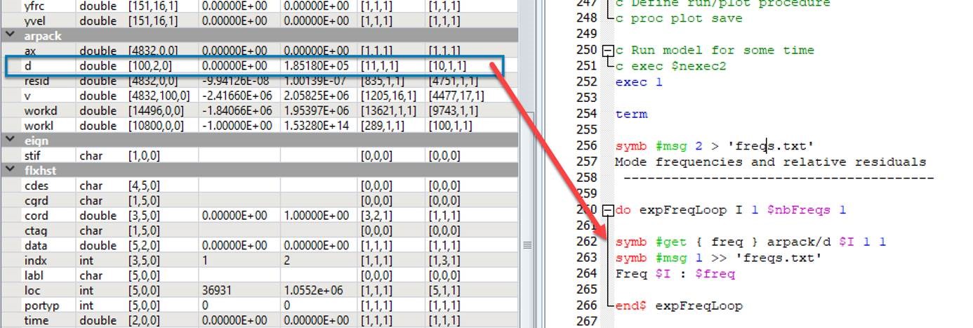
Note: The “symb #msg nb” command print to console the nb next code lines. If you add “ > filename.txt” it will save to a file instead. If you use “>>” it will append to the end of the file. You can then make a loop which find the frequency variable in the arpack/d array and save it into a variable freq
Limitations of the current modal solver
The current modal solver doesn't support viscous damping vdmp. Thus you can only calculate the modal shapes of a transducer without the water around it.
Make sure that you do not have the vdmp damping model in your material properties.