
In this tutorial we will learn how to set up a simple 2D model of a wave propagating in steel containing a defect using the designer mode primitives. We will make use of a symmetric shape and analyse only half of the model.
We will learn:
- How to set up a 2D Symmetric model
- How to assign a time dependent load
- How to create the 2D geometry using simple geometry shapes
- How to solve the model to calculate the acoustic pressure
Problem Definition
Characteristics of the model
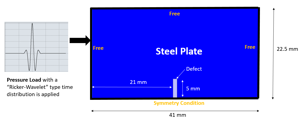
| Model: | Half Steel Plate of Dimensions 41 mm x 22.5 mm with a rectangular defect of dimensions 21 mm x 5 mm |
| Mesh Size: | 15 Elements / Wavelength |
| Analysis Time: | 5e-05 seconds |
| Output Results: |
- Time History of Acoustic Pressure at X= 20 mm - Maximum Acoustic Pressure Field |
Material Data
| Name | Mild Steel, Generic |
| Code Name | steel |
| Density | 7900 kg.m-3 |
| Bulk Velocity | 5900 ms-1 |
| Shear Velocity | 3200 ms-1 |
Note: Material Data in OnScale are generally defined using the bulk velocity and the shear velocity parameters instead of the more traditional Elastic Modulus and Poisson's Ratio. You can check this page if you want to understand the relation between those parameters.
Step by Step Tutorial in Video
Before analyzing anything more complex, the best is to understand the basics of how to simulate the propagation of an ultrasonic wave into a steel plate.
In a real Non-Destructive Testing Simulation project, you might want to do exactly the same thing than in this simple example, but with probably a geometry slightly more complex, that's why this tutorial is an extremely good tutorial for beginners of OnScale.
Imagine that the notch into the plate is a defect of your material that you cannot detect with bare eyes because it is too small. Such defect could cause a lot of problem if it appeared in very sensitive type of project such as the wing of an airplane for example!
Note: The Designer interface has changed slightly since this video was recorded. The text that follows has been updated to reflect the interface changes.
With simulation though, you get an extremely cheap way to look for this type of defect "virtually" and their impact on the overall structure of your material.
The Simulation Process
Step 1 - Creating a New Project
Before we begin we must create a new project.
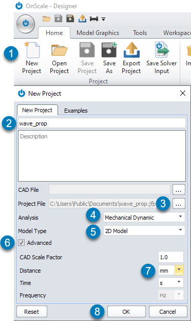
- In the Home tab of the ribbon, click New Project. The New Project window shows.
- Type a name for the project.
- If desired, change the save location and/or project file name by clicking … beside Project File.
- For Analysis, select Mechanical Dynamic.
- For Model Type, select 2D Model.
- Select the Advanced checkbox.
- For Distance, select mm.
- Click OK.
Step 2 - Adding the Materials
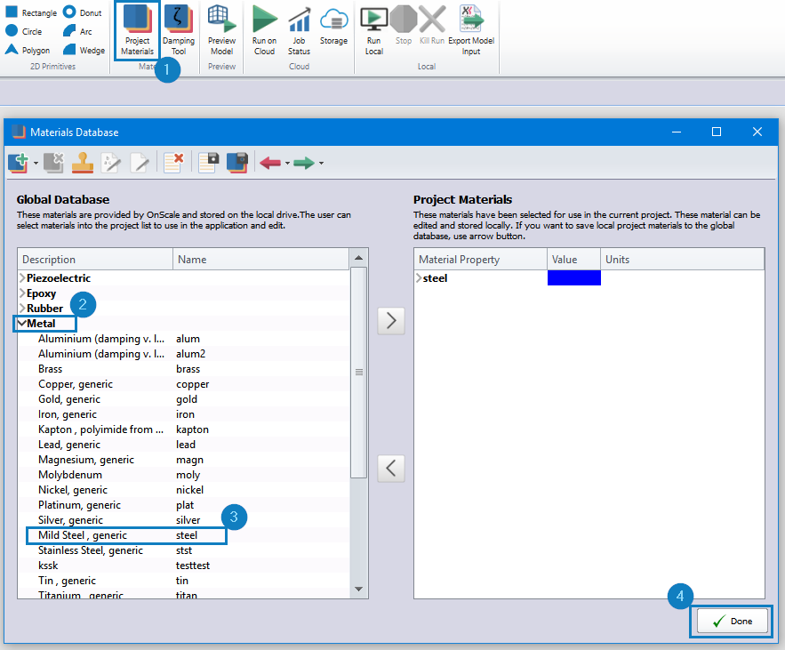
First we will add the materials needed from the material database. We will use Steel in this tutorial.
- Click Project Materials to open the Material Database
- Expand the Metal tab
- Double click 'Mild Steel, generic - steel' to add this to Project Materials
- Click Done to close the Material Database
Step 3 - Creating the Geometry
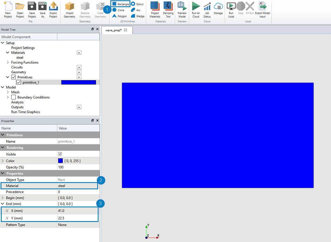
We will make use of the geometric primitives available in Designer. We will use the Rectangle primitive twice.
Creating the steel plate geometry
- Click to add a Rectangle to the workspace
- Change material to steel
- Set End (mm): X (mm) = 41 and Y (mm) = 22.5
Note: After making changes to X and Y right click the workspace and select Reset View
Adding the defect geometry
- Right click primitive_1 and select Duplicate Selection
- Click primitive_2
- Change material from steel to void
- Set X (mm) = 20
- Set X (mm) = 21 and Y (mm) = 5
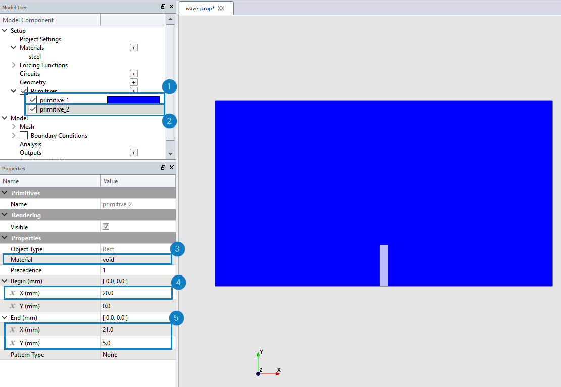
Important: In OnScale, you do not need to perform "boolean operations" and to cut the initial plate shape to add the defect, you can just superimpose basic geometry shapes on the top of one another and assign "void" as its associated material.
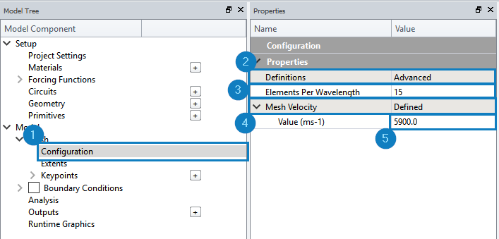
Step 4 - Setting up the Mesh
We will now change the mesh settings to use 15 elements per wavelength
- Select Configuration
- Set Definitions to Advanced
- Elements Per Wavelength = 15
- Expand Mesh Velocity - Click 'Min.Bulk Material Velocity' change to 'Defined'
- Set Mesh Velocity Value to 5900
Important: In order to get good and accurate results out of an acoustic simulation, the size of the grid should be chosen sufficiently small. We can calculate the best size of the grid required by calculating the wavelength of the vibration into the chosen medium. Once we have that, we know that we should choose a grid size of around that wavelength divided by 15 to get good results.
Step 5 - Creating a New Load
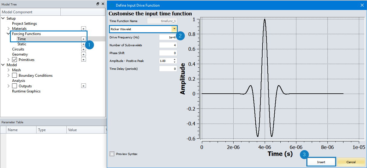
Adding a Time Function
The pressure load we will assign to our model will follow a "Ricker Wavelet" type of time distribution, so we need to add this specific time function in advance to our project to be able to associate it later on the load
- Click '+' to open the Time Function window
- Change Sinusoid Pulse to Ricker Wavelet
- Click Insert
Creating a Load
- In the Model Tree, expand Boundary Conditions and then, beside Loads, click +.
- For Creation Mode, select Geometry Interface.
- For Geometry, select primitive_1 (steel) or click it in the model.
- For Interfacing Item, select side 1 (xmin).
- Click Create Load.
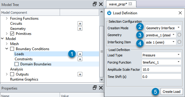
Upon clicking Create Load a record load_1 will be added to the Model Tree after this you can close the Load Definition window.
Step 6 - Setting up Boundary Conditions
We will need to change the Y minimum boundary condition to Symmetry as this model is symmetrical along that axis.
- Click Domain Boundaries
- Change the Y Minimum boundary condition to Symmetry. Leave all others as default.
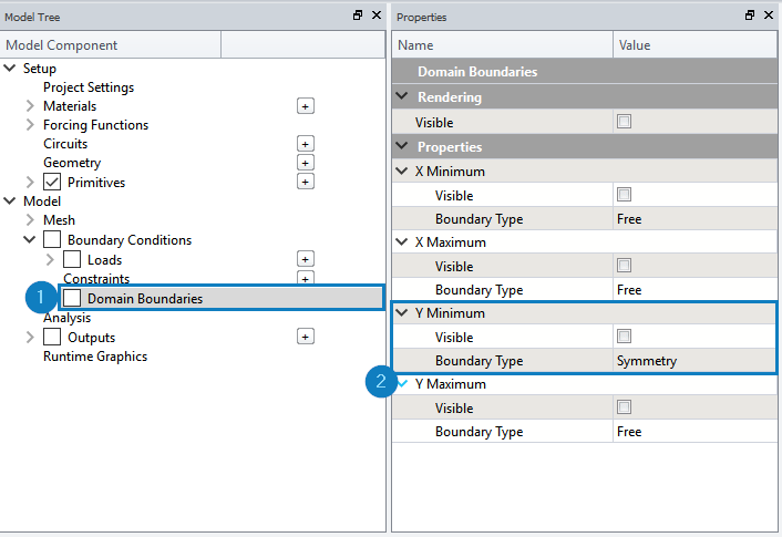
Note: Boundary conditions in this case are set up globally to the maximum and minimum edges of the model both in the X direction and in the Y direction. In you want, you can also set boundary conditions individually by adding some "constraints" to your model.
Step 7 - Setting Analysis Time
We will now set the model simulation time to be 5e-5 seconds
- Click Analysis
- Set Simulation Run Time (s) to 5e-05
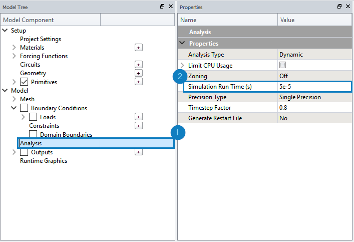
Important: Choosing an appropriate analysis time is critical for the analysis! Make sure your analysis time is not "huge" in comparison with the velocity of propagation of the wave into the medium otherwise your simulation will take ages to complete.
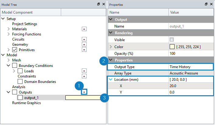
Step 8 - Choosing Output Results
We will now define 2 outputs, a time history of the acoustic pressure on the front of the defect will be recorded and the maximum pressure array will be outputted
Note: In OnScale, all the calculated results have to be defined in advanced before you start the simulation, otherwise they will not be calculated. Make sure you set up all the results you are interested in to avoid having to run the simulation more than necessary.
Time History of Acoustic Pressure at X= 20 mm
- Click '+' this will create a new output
- Change Output Type to Time History
- Set Location (mm): X = 20
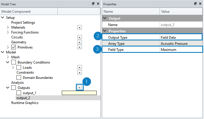
Maximum Acoustic Pressure Field
- Click '+' this will create a new output
- Change Output Type to Field Data
- Change Field Type to Maximum
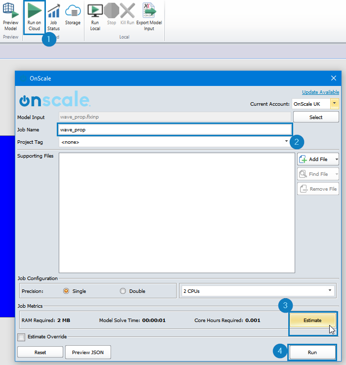
Step 9 - Launch the simulation on the Cloud
At this point the model is completely set up and it can now be run on the cloud.
- Click Run on Cloud
- The option to rename your job. This is how it will appear in the storage
- Click Estimate
- Click Run
Step 10 - Post Processing Simulation Results
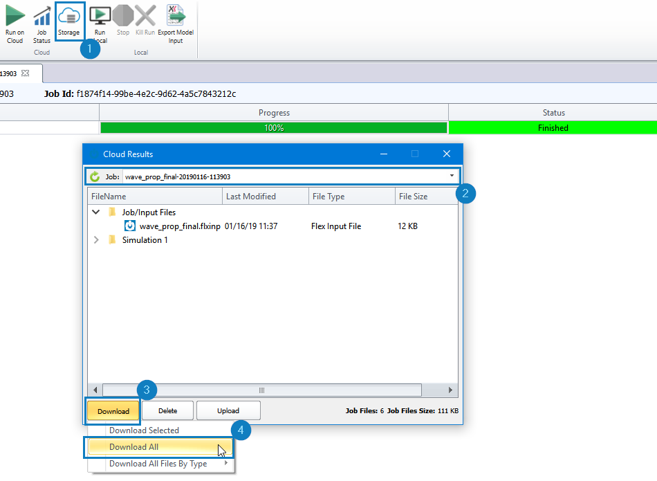
Download the results from the cloud
The simulation results will need to be downloaded from the cloud storage in order to analyse the results in the post processor. More experience users may also be able to process Time Histories in Review.
- Click Storage this opens the window shown above
- Locate the job
- Click Download
- Click Download all
Choose an appropriate save location when the file explorer pops up and click Select Folder to close the window.
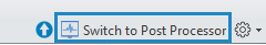
Switch to the Post Processor
Important: Once you downloaded the results from the cloud, those results will be available on your computer locally. You will then need to open them into the post-processor to visualize them.
Click this icon to access the Post Processor.
Open Results
- Click File Explorer
- Expand the job simulation folder. Open the flxdato file and the flxhst file (double click them)
- Click Results Manager
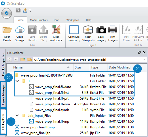
Note: Only the results displayed with gray icons *.flxdateo and *.flxhst can be opened into the post-processor.
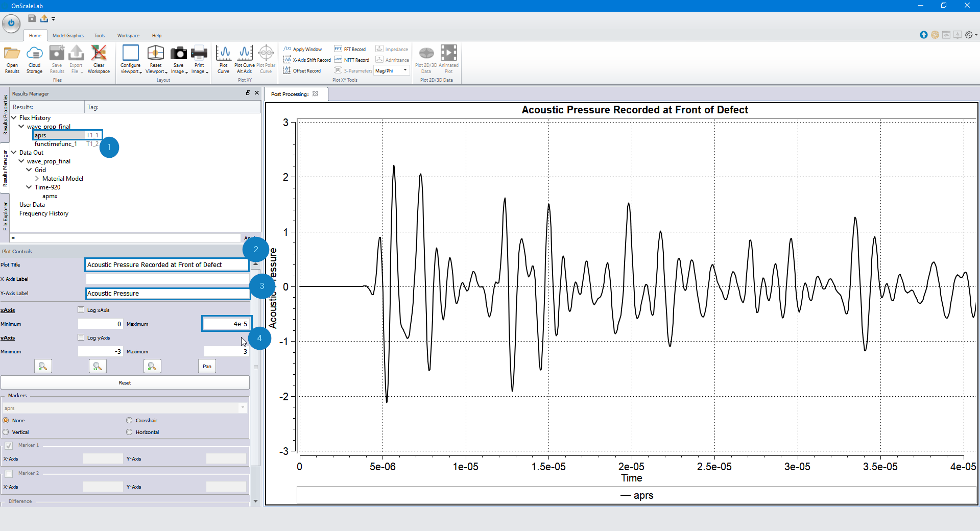
Plot Time History
Note: aprs = "Acoustic Pressure"
- Double click aprs to plot acoustic pressure
- Set plot title to Acoustic Pressure recorded at Front of Defect (optional title)
- Acoustic Pressure
- Change Maximum value to 4e-5
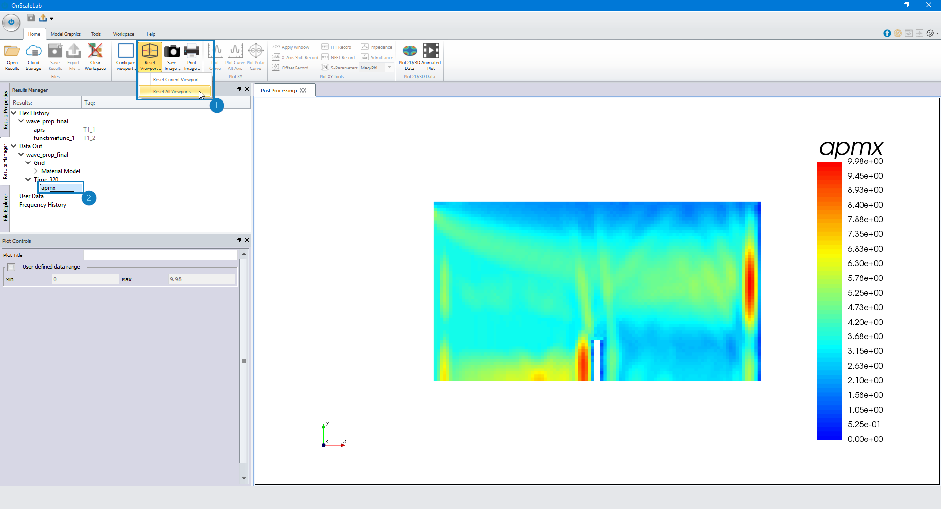
Plot Data Array (Maximum Pressure)
Note: apmx = "Acoustic Pressure Maximum"
- Click Reset Viewport and choose Reset All Viewports
- Double click apmx to plot the maximum pressure data array
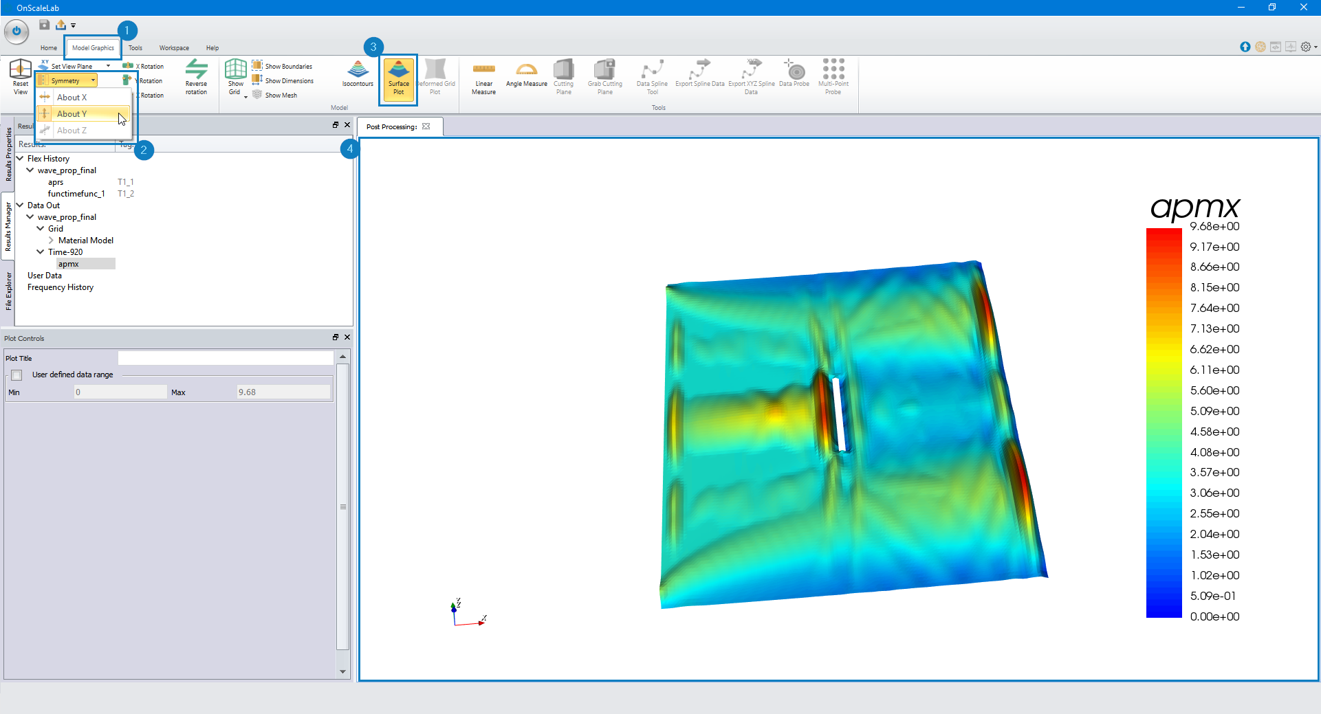
Displaying Surface Plot
- Click Model Graphics
- Apply Symmetry about the Y axis
- Click Surface Plot
- Click the workspace and move to rotate the model
Try for yourself
Now that we have introduced you to the tutorial try have a play around with some of the settings, add some other outputs, or use this model as a starting point for your own.