Acoustic wave propagation in multi-layered structures is used in different industries for numerous measurements, evaluation and imaging applications. Technology based on this method is used in the Oil and Gas industry to characterize underground reservoirs during their entire life cycle; starting from exploration to their abandonment. This technology is referred to as Borehole Acoustic Measurement (Logging) and is further classified in to Sonic and Ultrasonic Logging
Sonic Logging Principle
Borehole Sonic Logging is based on the principle of measuring the travel time of Compressional (P), Shear (S) and Stoneley waves propagating along a borehole with different radial depths into the formation. The operating frequency range for these measurements is typically from 0.5 to 20 kHz. This helps to probe several meters into the formation. In this tutorial we will show you how to set up a sonic logging model and run it on the cloud.
The Model
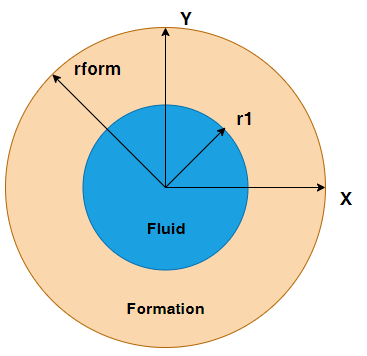
The model we will show you how to build today will be a fluid-filled borehole surrounded by a fast or slow formation. A formation is characterised as fast or slow depending on whether its shear wave velocity is slower or faster than the compressional wave velocity in the borehole fluid.
The sonic measurement tool or in this case the pressure wave excitation will be located at the centre of borehole, the receivers will also be located along the centre of the borehole the first receiver will be placed 1.219m from the transmitter this will be referred to as the Tx-Rx spacing and the receivers are spaced periodically ever 0.152m the Rx-Rx spacing.

Download: 2D Sonic Logging Model
Step 1: Define variables
We need to define the following variables:
- Borehole & formation radii
- Height of borehole and sonic tool
- Tx-Rx and Rx-Rx spacing
- Mesh settings
Using the height of the sonic tool and the spacing variables you can calculate the number of axial receivers. The following inputs that we use will yield a total of 24 receivers.
Below is the code - it can be copy and pasted directly into a new Analyst script.
c ****************************
c MODEL INPUTS
c ****************************

c All inputs should be in this section
symb r1       = 0.13                /* open hole radius
symb rform    = 6 * $r1             /* formation radius estimate
symb h1       = 6                   /* height of borehole
symb h2       = 5                   /* height of sonic logging tool
symb hs       = 0.5 * ( $h1 - $h2 ) /* start of the tool (equidistant from top & bottom)
symb hr       = 0.285 - 0.152       /* location of last receiver on the tool
symb tr       = 1.219               /* transmitter to 1st receiver spacing
symb rr       = 0.152               /* receiver to receiver spacing

symb nr       = ( $h2 - $tr ) / $rr /* no. of axial receivers
symb ncopy    = $nr - 1

c read material properties
symb freq     = 5e3
symb freqdamp = $freq

/* Mesh settings
symb wlen = 1500 / $freq
symb nele = 40
symb boxy = $wlen / $nele
symb boxx = 3.25e-3
symbx ncycles = 50

/* Simtime variables
symb simtime = $ncycles / $freq
symb nloops = 100
Step 2: Keypoints and Grid
It is beneficial to set up the grid using keypoints to allow for rapid parameterisation and specific control of the model. We won't go into great detail in this tutorial about keypoints but check out this article for more information on keypoints and why you should be using them.
The symbol code has a number of #key options that allow for a quick method of generating XYZ and IJK model keypoints these commands also help to parameterise the model grid generation to allow for quick changes to the model geometry to be made. We will use the #key commands #keyindx and #keycord you can find more information on these commands in this article. We will also make use of the #key command #keycopy which allows for quick replication of already defined keypoints we will use this to create keypoints for each of the receivers along the borehole axis.
This code can be copy and pasted directly into the analyst script
c Keypoints
/* #keycordt allows XYZ keypoints to be generated from absolute dimensions instead of the distance between keypoints like #keycord
symb #keycordt x 1 0 $r1 $rform
symb #get { idx } rootmax x                /* store interger suffix of last keypoint
symb #keyindx i 1 $idx 1 $boxx 1

symb #keycord y 1 0 $hs $hr $rr            /* bottom of borehole to first receiver
symb #keycopy y 3 4 $ncopy                 /* copy keypoints 3 & 4 out ncopy times
symb #get { jrend } rootmax y              /* store interger suffix of last keypoint
symb #keycord y $jrend $y$jrend $tr $hs    /* finish keypoints in y starting from end of keycopy
symb #get { jdx } rootmax y                /* store interger suffix of last keypoint
symb #keyindx j 1 $jdx 1 $boxy 1

/* integer suffix to another variable
symb indgrd = $idx
symb jndgrd = $jdx

/* define the number of nodes in the computational grid, the number of dimensions for the model, and the appropriate constraint relations.
grid $i$idx $j$jdx axiy

/* To define nodal coordinates for the model.
geom keypnt $idx $jdx
Step 3: Defining Materials and assigning them to the grid
OnScale has a material database with a number of common materials readily available for users to use however for this tutorial we will need to manually define the fast and slow formations using the material properties shown in the image above. First though we will use the material database to save water to a file and we will edit that file. Save the file to the same working directory as the flxinp file.
- Expand fluid section
- Double click watr to add this material to the Project Materials
- Right click watr and select Copy - Call the new material watr2
- Click Save to File - save the file as sonic_logging_mat.prjmat
We have created a copy of watr to act as an interface to define a pressure load when it gets to that point
Once you have saved the file open it in the OnScale application add the following lines of code starting on line 58 of that file
/* fast formation
 wvsp on
 type elas
 prop form_fast 2350 3658 2032 0.01

 /* slow formation
 wvsp on
 type elas
 prop form_slow 2054 1890 508 0.01

 /* anisotropic material properties
 wvsp off
 type lean
 prop form_aniso 2350
 23.87 15.33 9.79 0 0 0 23.87
 9.79 0 0 0 15.33 0 0
 0 2.77 0 0 2.77 0 4.27
Now that materials have been defined we can now assign those materials to elements of our grid to do this we use the SITE command. This is where keypoints come in handy because now we can define regions between start and end keypoints in a given direction to assign material to all the elements encapsulated by that window.
The code can be copy and pasted directly into the analyst script you are working with
c **************************************************
c MATERIAL PROPERTIES
c **************************************************
symb #read sonic_logging_mat.prjmat

site
     regn void                       /* All materials must be assigned a material initalise them all with void
     regn watr $i1 $i2 * *           /* Assign water to borehole region
     circle2d watr2 $x1 $y28 0.01    /* 1 element defined as watr2 to define an interface to apply a load to
     regn form_slow $i2 $i$idx * *   /* assign fast material to formation region

grph
     nvew 2 2                        /* create two plotting viewports
     plot matr                       /* plot geometry
     mirr x on                       /* turn mirror on x-axis to show full representation of half symmetry models
     plot matr                       /* plot geometry with mirror conditions on
term

Step 4: Boundary Conditions and Loads
It is best to simplify the model as much as possible. If you are modelling a symmetrical object and the same conditions are applied to both sides of the model, there is no reason to model the entire structure. It is more efficient to model half (or less) of the structure and achieve the same results for a fraction of the computing time. We will apply a symmetry boundary on the minimum X extent of the grid. For more information on the topic of boundary conditions check out the following articles:
How to Apply your Own Boundary Conditions
IMPD (Impedance) vs. ABSR (Absorbing) Boundary Conditions
We will also apply a pressure load on the interface of the materials watr and watr2 this will act as a monopole pulse we will also provide you with the text file that contained the time and amplitude values of the pulse we used.
c External boundary conditions
boun
 side xmin symm
 side xmax impd 2350 3658 2032
 side ymin absr
 side ymax absr

c Define time varying funciton
data hist pulse * pulse_5kHz.txt    /* open the text file and save it to an array called pulse
func hist pulse                     /* assign array to a time history func

plod
     pdef pld1 func                  /* create pressure definition and specify function to be used
     spot spt1 $x1 $y28              /* defining the side of a surface to which a normal pressure loading will be applied
     sdf2 pld1 spt1 watr2 watr       /* surface is defined as the interface between two material regions of the model
Step 5: Calculations and Outputs
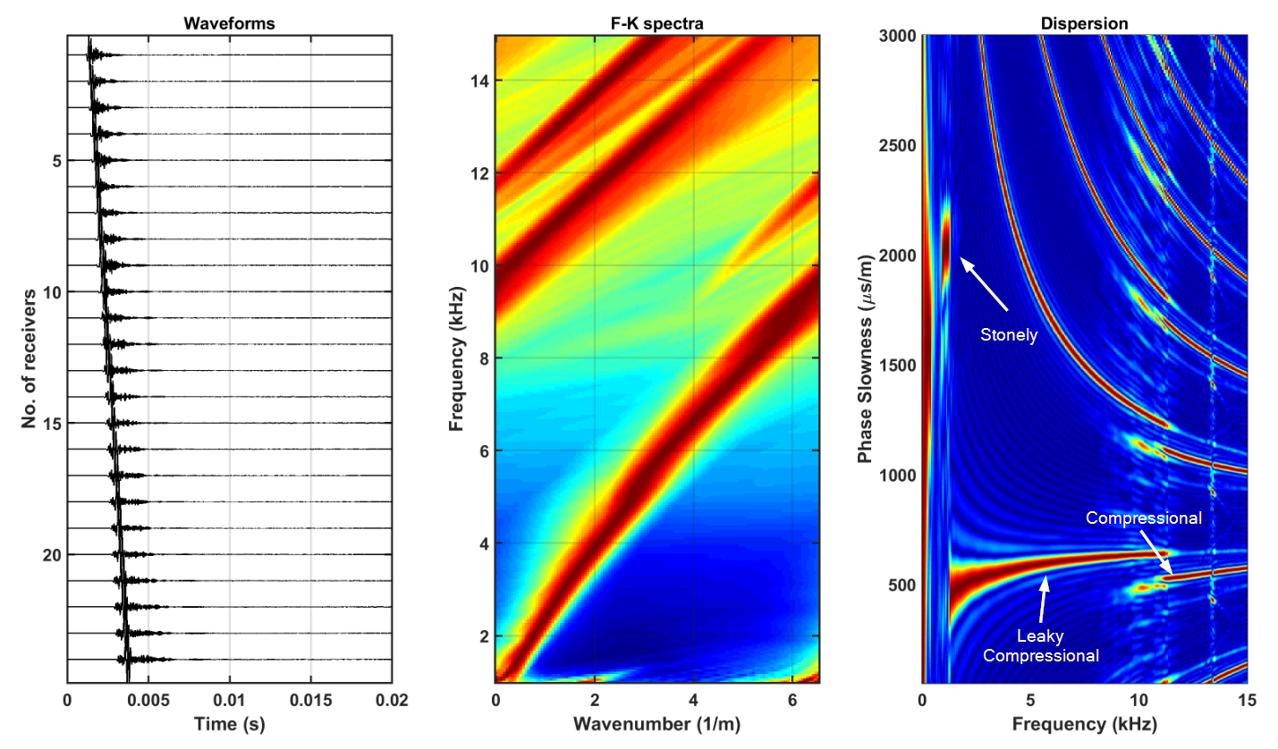
The receivers situated on the borehole axis measure the time it takes for the acoustic pulse to travel in the formation in various forms while undergoing dispersion and attenuation. When the sound energy arrives at the receiver, having passed through the formation, it does so at different times in the form of different types of waves. This is because these waves travel with different velocities we want to capture these waveforms so we need to set up outputs to capture the acoustic pressure measured on each receiver
c Request calculation of additional arrays
calc pres aprs                           /* open an additional APRS array - acoustic pressure

c Request time domain outputs saved to a flxhst file
pout
     hist func                           /* write function to a output file
     symb jrx = 3                        /* keypoint suffix of first receiver
     do loop_rx J 1 $nr 1                /* open do loop to loop through receivers
        hist aprs $i1 $i1 $j$jrx $j$jrx  /* loop through receiver locations to output acoustic pressure at these points
        symb jrx = $jrx + 1              /* add one to the keypoint suffix
     end$ loop_rx                        /* close loop
Step 6: Process and Model Execution
Before running the model, you should always issue the prcs command. In preparation for processing the time-step information, it computes the model time step for stability and opens the necessary arrays for field-data storage.
The basic information required prior to executing the model:
- Model timestep (step)
- Simulation runtime (simtime)
- Simulation runtime in terms of number of timesteps (nexec)
c ***********************
c PROCESS MODEL
c ***********************
c Time settings
time * * 0.8

c Process model
prcs

grph
     set imag mpeg                                /* set to generate a video
     nvew 1
     mirr x on

c ***********************
c MODEL EXECUTION
c ***********************

symb #get { step } timestep                       /* extract calculated timestep from prcs command
symb nexec_loop = ( $simtime / $step ) / $nloops  /* partition full simulation into smaller segments for plotting

c Runtime calculations
proc exec_loop save                               /* name procedure exec_loop and save the code
exec $nexec_loop                                  /* run model partially
grph
     mirr x on
     plot aprs rang 0                             /* plot acoustic pressure - shows wave propagation
     imag

end$ proc                                          /* end of procedure

c run model by calling 'plot' procedure 'nloops' times
proc exec_loop $nloops

c Save symbols to file for later use
symb #get { labl } jobname                         /* find name of run
symb #save '$labl.symb'                            /* save in symb file

c End of input file
stop
Step 7: Running the model on the cloud and downloading the results
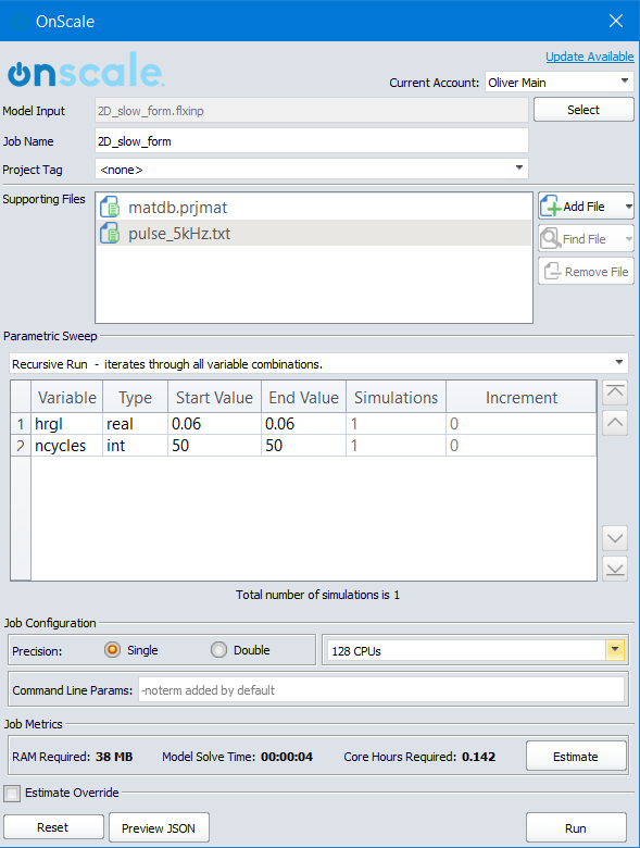
Now that the models have been set up they can now be ran on the cloud - To do this simply open the cloud scheduler (Run on Cloud ![]() ) and click the estimate button once the estimate is completed you can click run and this will spool up hardware on the cloud and submit your files.
) and click the estimate button once the estimate is completed you can click run and this will spool up hardware on the cloud and submit your files.
Once the simulation is complete if you click the storage icon to open the cloud storage - after a simulation this is where the results are stored you will have to download them first before you can do anything with them. To access the storage click  locate the job you have just run and download the results.
Step 8: Post-Processing the Results
We post-processed all of our results in MATLAB, we can provide a MATLAB script that we used. This is not a MATLAB tutorial however so there will be no instructions from here on out but here is a what the processed results look like if the script is used correctly.