
Monte Carlo Simulation a statistical method which uses simulation to model the probability of outcomes of a complex model whose behavior cannot be easily determined due to a vast number of variables.
In this example we vary three parameters of a curved waveguide: core width, core thickness and inner bend radius and analyse the effect on transmission coefficient.
Model Setup
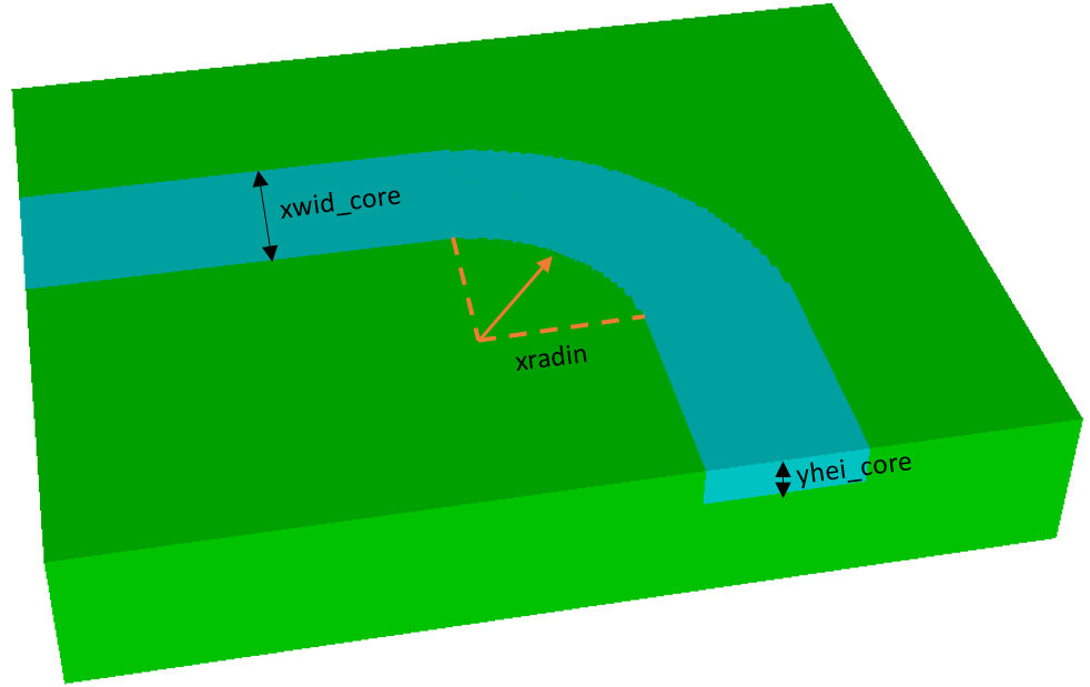
A schematic of the model and the three input variables can be seen below:
The key model parameters were as follows. The variables to be randomly varied are indicated by *
| Design Variable | Description | Default Value |
|---|---|---|
| xwid_core * | Width of core | 1500 nm |
| yhei_core * | Thickness of core | 800 nm |
| xradin * | Curved section's inner radius | 1700 nm |
| yhei_model | Total thickness of model | 3000 nm |
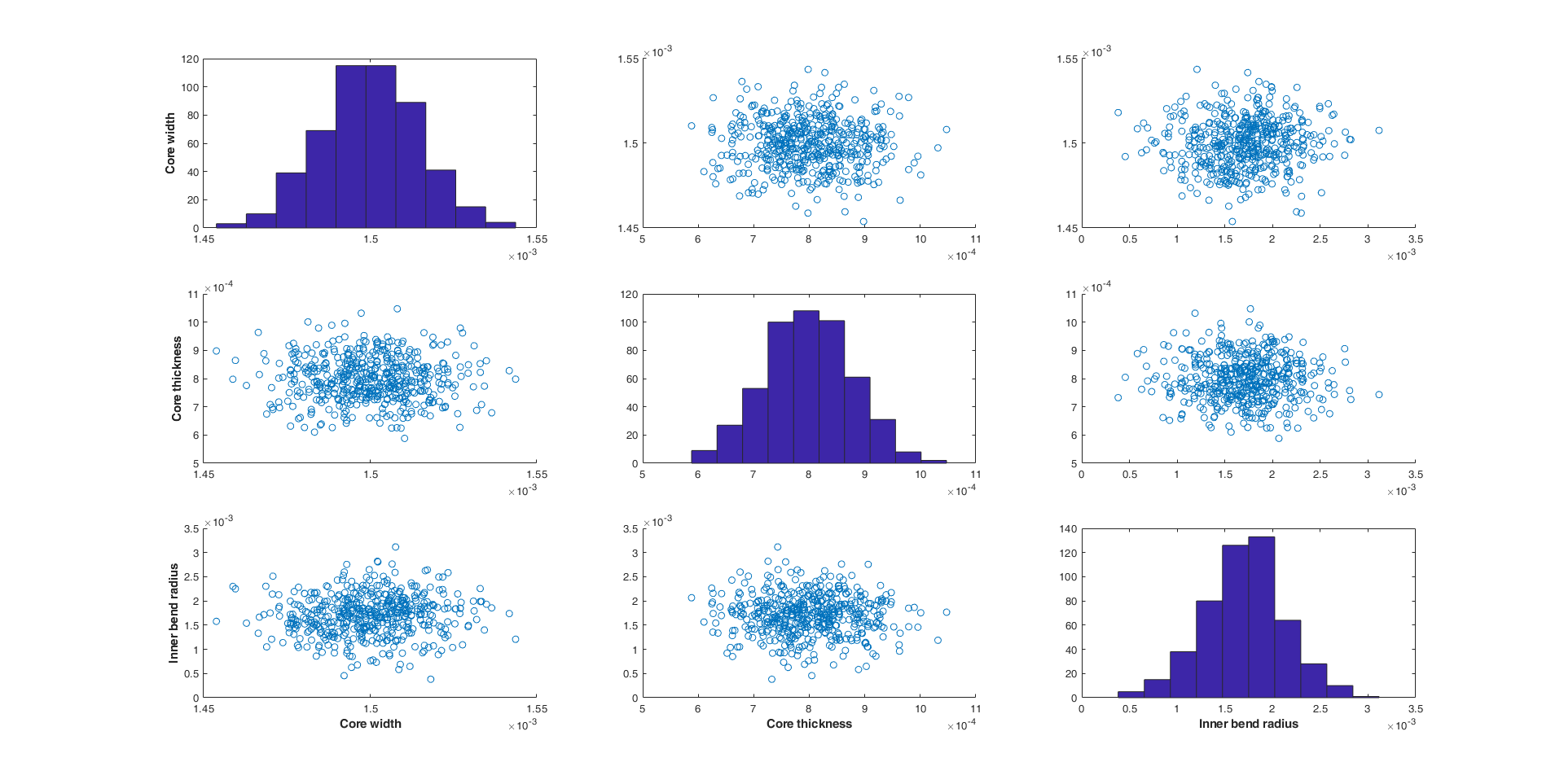
500 random input variables were created with the following constraints:
- Core width: 1500 nm ± 10%
- Core thickness: 800 nm ± 10%
- Inner bend radius: 1700 nm ± 25%
Monte Carlo Results
The full study was completed in 7 minutes when using 2 cores per simulation and had a total cost of 76.28 Core-Hours.
The transmission coefficient was calculated using the power in and out of the waveguide. To see the affect the four parameters had on transmission coefficient results are plotted below in MATLAB.
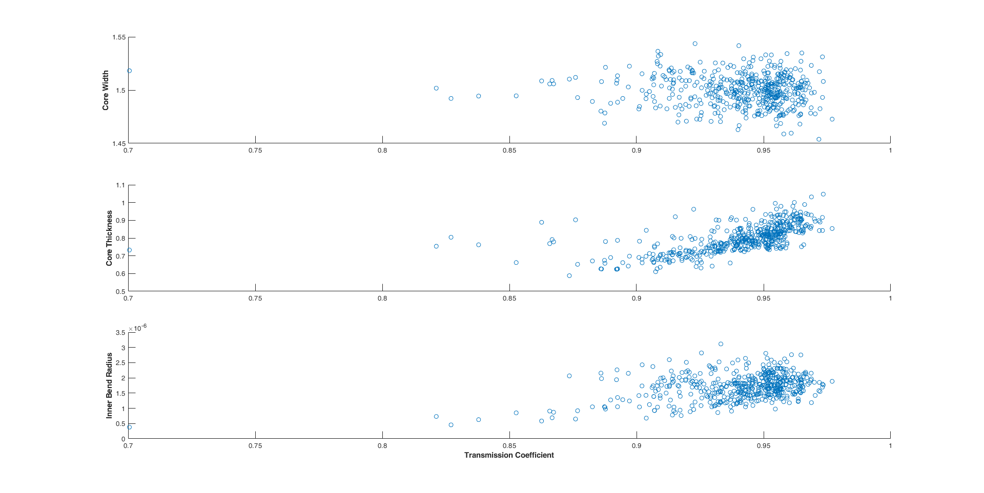
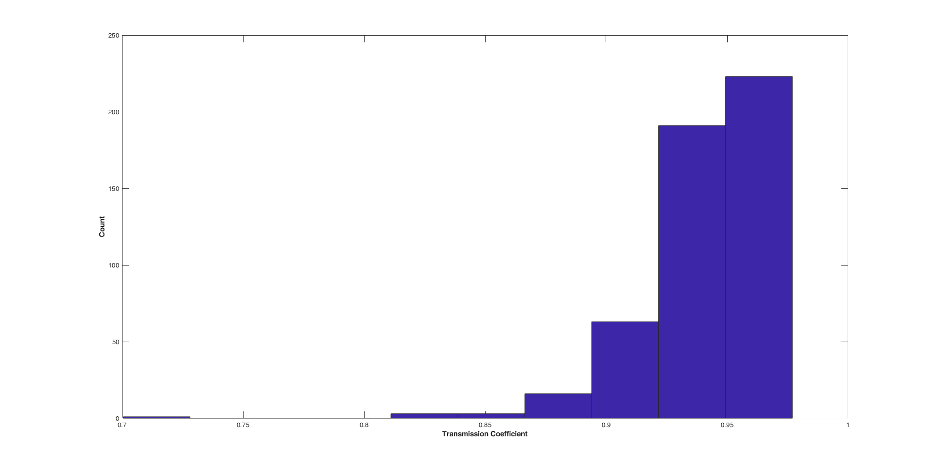
The Monte Carlo study shows that there is a spread of transmission coefficients between ~70% and ~97.5% with more being on the higher end of that scale. The study also shows there is a direct correlation between core thickness and transmission as well as inner bend radius and transmission.
Try this Yourself
To run this Monte Carlo study you will need to download the OnScale and MATLAB files.
- Extract all of the files from the downloaded folder
- Open 'monte_carlo_pre_v1.m' and select run
- Open OnScale and Select Cloud Scheduler
- Select 'curved_SOI.flxinp' as the input file
- Under Parametric Sweep, select User Defined Variable File from the dropdown
- Next to Input Files, select ... and open 'simdata.csv'
- Select Estimate + Run
- Download all *.symb files
- Open 'trans_coeffs.m'
- Insert the name of results folder that was downloaded into the variable FIn
- Select Run
- Open 'monte_carlo_post_v1.m' and select Run