General Use
Free field (ffld) boundaries are for splitting large models into two stages where one of the stages is altered while the other remains the same. This greatly reduces the simulation times for running variations of either stage of the model.
The most common way to think about this type of problem is saving pressure time histories in one simulation, then using them as input to another, related simulation. Issues will occur with this approach as the impedance at the absorbing boundary condition will not match the second simulation.
Note: Caution will need to be used in ‘stitching’ the three simulations together here. Boundary conditions of each successive one will have to match the co-ordinate range of the previous simulation. Some care has to be taken if changing mesh density too.
A simple example can be found here:
The ffld command works with both acoustic and elastic waves. It can be used to couple both 2D plain strain and 2D axisymmetric simulations into 3D.
Note: If applying in axisymmetry the user will have to use a cyln coordinate system.
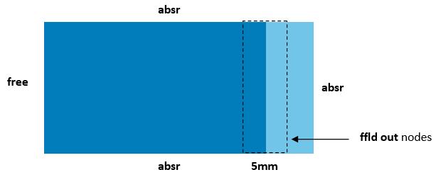
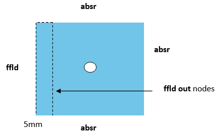
It will interpolate points if grids are mismatched. Again, care must be taken to make sure center elements are accounted for in new grid. This means the ffld out region must span at least 2 elements. This is to ensure stresses can be calculated correctly, important if applying the stnd condition i.e. ffld and absr boundary is used.
If problems still persist in matching up the coordinate systems, the ‘fuzzfactor’ can be increased to provide more tolerance for connecting mismatched nodal positions between grids.
Common applications where this will be useful:
- Acoustic Microscopy
- NDE
- Any pulse-echo or reflection situation where either target or source can varied independently.
The time command can be used in models where the ffld condition is loaded and users do not wish to execute from 0.0 seconds, but at a more suitable start time to avoid initial ‘wait’ time for the ffld to arrive.
Model Example:
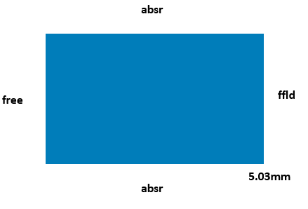
- Source and receive models have same height
- Target model is smaller than the send and receive models to ensure stresses can be interpolated
- Mesh is even in both X and Y
- Same meshing except there is increased mesh density in target model to better resolve ‘defect’.
Source Model - 15 Element per Wavelength
Target Model - 30 Element per Wavelength
Receive Model - 15 Element per Wavelength